Multidimensional Scaling Outlier Detection - With a Real-World Example
Attachments: article_data.txt
Sections
Multidimensional scaling (MDS) is a machine learning algorithm for converting high dimensional data points into lower-dimensional ones while preserving the distance between them as much as possible. A common use for this is for visualizing a set of high dimensional data in two or three dimensions.
Feature engineering combined with MDS is one of my bread-and-butter methods for outlier detection. In this article, I will briefly go through the version of MDS that I use and a real-world example of how I used it to find outliers in a project.
Metric MDS
Suppose we have a set of high dimensional data points \( X = (X_1, X_2, \dots, X_n) \), where each point \( X_i \in \mathbb{R}^n \) for some large \( n \). There are several versions of MDS that have the same objective of taking the data points in \( X \) and projecting them onto a lower-dimensional subspace while preserving the distances between them as much as possible.
I am just going to focus on a particular version known as metric MDS. In general, MDS algorithms operate on the dissimilarity matrix \( D \), where \( d_{ij} \) is a number that quantifies the dissimilarity between data point \( X_i \) and \( X_j \). For metric MDS, \( d_{ij} \) must satisfy the mathematical criteria of being a metric distance. Thankfully, the usual Euclidean distance satisfies those requirements. \( D \) is then known as a metric distance matrix.
Metric MDS then tries to find a set of points \( Y = (Y_1, Y_2, \dots, Y_n) \) in a lower dimension \( \mathbb{R}^m \) that we specified. Usually, \( m = 2 \) is chosen so we can use a 2D scatter plot to visualize the dataset. \( Y \) is found by minimizing a cost function called stress.
From the \( ( d_{ij} - \lVert Y_i - Y_j \rVert )^2 \) term we can see that the algorithm is trying to find a set of points \( Y \) so that the Euclidean distance of every pair of points \( Y_i \) and \( Y_j \) are as close as possible to the original distance between \( X_i \) and \( X_j \).
While gradient descent can be used to find an approximate minimum for this loss function, it is surprisingly not used for metric MDS. Instead, an interesting algorithm called stress majorization is used. It is too complicated to describe here, but the rough idea is that there is a function that bounds the stress function from above. Then, an iterative process will keep tightening this bound until it reaches a value we are satisfied with.
One important thing to note about metric MDS is that because the input is a metric distance matrix, the algorithm is sensitive to the units of your original dataset \( X \)! For example, if the first coordinate in every vector \( X_i \) is several orders of magnitude larger than all the rest, it would dominate when calculating distances.
Real World Example
This is a real-world example of how I used feature engineering and then metric MDS for an outlier detection project. The data has been heavily modified, and the context will be kept vague. Whether it still reflects the actual real-world use case will have to be a “trust me, bro” situation! Also, there are many ways to do outlier detection, and this is a description of just one particular way of doing it that I find to be extremely useful.
Feature Engineering
The Wikipedia page for anomaly detection defines it as:
Identification of rare items, events or observations which deviate significantly from the majority of the data and do not conform to a well defined notion of normal behavior.
With this definition, we can already imagine what this will look like in a 2D scatterplot generated by metric MDS: a clump of closely located data points representing the majority of the data with normal behavior and a few outlier points far away from this clump.
What I like to do is to think about what kind of outliers the end-user or client is trying to find. There are countless ways to define what an outlier is. Which ones would be meaningful to them? Then, I do feature engineering to generate features that I know will help in finding the kind of outliers that will meet my client’s business objectives. Of course, knowing what the potential output of machine learning models will be requires a little bit of experience!
For this project, I came up with four features. The \( n = 1,886 \) data points’ features can be found in the article_data.txt file in the attachment section at the top of this article. We will be using this file for the next subsection. Also notice that these features have been normalized because metric MDS is not unit invariant.
Metric MDS
Metric MDS can be easily done with the well-known scikit-learn package in just a few lines of code.
 1import pandas as pd
 2from sklearn.manifold import MDS as mds
 3from matplotlib import pyplot as plt
 4
 5data = pd.read_csv('article_data.txt', header=None)
 6embedding = mds(n_components=2, n_init=1)
 7transformed = embedding.fit_transform(data)
 8
 9plt.figure(figsize=(8, 8))
10plt.scatter(transformed[:, 0], transformed[:, 1], cmap='viridis', s=50)
11plt.grid(True)
12plt.show()
The output is a projection of the \( n = 1,886 \) data points from the four-dimensional space of the four features onto two-dimensional space while preserving the original four-dimensional distances as much as possible. Note that the algorithm is not deterministic and has a random output. So, you might get a different figure from the one I got below.

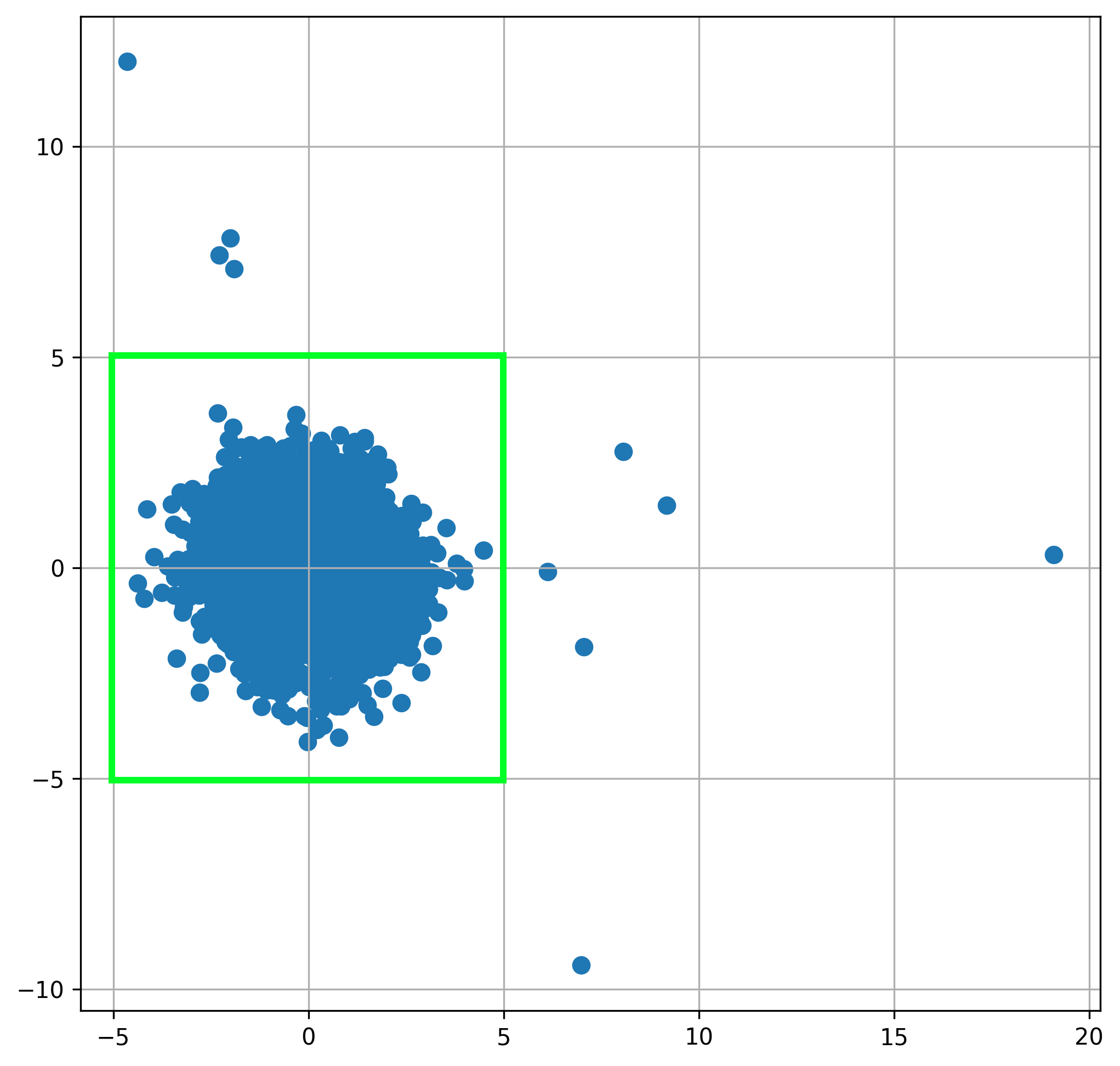
We can set simple rules for which data points to flag as outliers.
-
Draw a green box with \( (x,y) \) coordinates \( -5 \leq x \leq 5 \) and \( -5 \leq y \leq 5 \).
-
Data points within the green box are considered normal.
-
Data points outside the green box are considered outliers.
The figure below shows what these rules and the ten outliers they singled out will look like in our plot.
Note that there is no mathematical definition of what is an outlier. It is completely subjective and depends on what the client’s business objectives are!