Attention Is All You Need
The Attention Mechanism in Recurrent Neural Networks
Sections
- Feedforward Neural Networks
- Sequence Data
- Recurrent Neural Networks
- Encoder-Decoder Configuration
- The Attention Mechanism
If you are reading this, you probably know about the infamous Attention Is All You Need paper. This article talks about the recurrent neural network (RNN) and attention mechanism that are described in the introduction section of the paper.
In my humble opinion, this is the absolute best way to learn what the attention mechanism is and what the paper is trying to do. After all, the key breakthrough of the paper is a paradigm shift of that industry standard RNN + attention setup, where they realized they don’t actually need the RNN!
Feedforward Neural Networks
The classic feedforward neural network tries to solve this problem: given an input \( x \), produce an output \( y \) that reflects what we see in the data as closely as possible. One reason to do this is if we want to “predict” the corresponding \( y \) to a given input \( x \). Note that both \( x \) and \( y \) could be vectors and not just real numbers.
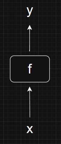
A function \( f \) can be implemented using a feedforward neural network to take in \( x \) and produce the output \( y \).
The figure below is how I would visualize a simple feedforward neural network.
To do this, we need to “train” the neural network \( f \) on a set of training data \( \{ (x_1, y_1), ..., (x_n, y_n) \} \). This just means tweaking the parameters of \( f \) so that for a given input-output pair in our training data \( (x_i, y_i) \), we have
“\( \approx \)” represents some vague notion of “close enough”. Usually, the parameters of \( f \) are tweaked and judged as “close enough” based on some loss function.
Sequence Data
Recurrent neural networks (RNNs) were made to solve a similar problem, but with one key difference: what if the input and output are sequences, and we want to incorporate the sequential information?
Let me explain what this means. Technically, the input \( x \) and output \( y \) in the previous section can be vectors. However, the entries in these vectors are not assumed to have any structure or be related to each other.
For example, suppose we have \( y = a \oplus b \), where \( \oplus \) stands for exclusive or. Then, \( a \) and \( b \) could be independent random variables. But we can still define the input as \( x = (a,b) \) and construct a feedforward neural network \( f \) such that
Just remember to avoid using a perceptron for \( f \) and you should be fine most of the time.
When we say the input and output are sequences, we mean that there is a notion of \( a \) coming before \( b \) in the vector \( x = (a,b) \). To make it easier, I am going to use capital letters to denote the sequences and lowercase letters to denote elements within the sequences.
For example, \( X \) could be a sentence, and each entry \( x_i \) is a word in the sentence. Then, the fact that \( x_1 \) follows from \( x_0 \) in the sentence has significance most of the time. For example, there is a big difference whether the word “not” appears before the phrase “a cat”! Or \( X \) could be a time series of prices for a stock over \( n \) days. How the stock behaves in the past could be significant information.
Recurrent Neural Networks
We could treat these two sequences as vectors and do the same as before, using a feedforward neural network \( f \) to produce an output sequence \( Y \) from an input sequence \( X \).
But this might feel like throwing away potential information contained within those sequences. Note that, as far as I know, there is no mathematical proof that we are indeed throwing away information. Also, there is no proof that recurrent neural networks (RNN) retain all possible information about sequences. There might be other, better ways to handle sequences. It is very much based on vibes!
Let’s start with a simple input sequence,
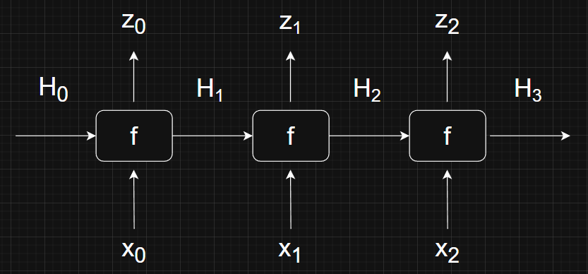
The idea behind RNNs is to start with the first element \( x_0 \) and a vector \( H_0 \). The vector \( H_0 \) is known as the hidden state and can be initialized with all zeros. Then, have function \( f \) produce an output \( z_0 \) and hidden state \( H_1 \). This process is repeated for each element in the sequence, using the hidden state produced during the previous step as input to the next step.
I would visualize this process like this.
Next Token Prediction and Hidden States
You might be wondering what the output \( z_i \) are for? We can think of them as a prediction of the most likely element that will appear after our input element, similar to how large language models (LLMs) do next token prediction. The LLM connection shouldn’t be a surprise since the Attention Is All You Need is precisely an evolution of the classic RNN next element/token prediction paradigm!
What about the hidden state \( H_i \)? This is how RNNs choose to retain information of what came before in the sequence. At each step, \( H_i \) works like some kind of memory that stores all the information of elements that came before \( x_i \). Again, I need to emphasize that this is just one way of carrying information about past elements into the future and need not be the only or best way.
Compact Representation
Instead of writing out each step explicitly, we can write the entire process as
Similarly, we can visualize the RNN more compactly like this.
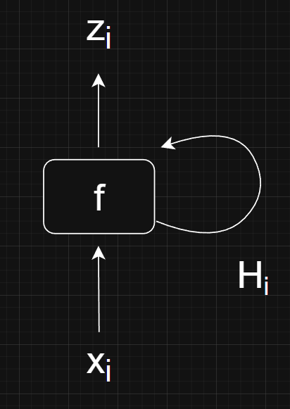
Although I think this version of the diagram is more confusing and less enlightening.
Encoder-Decoder Configuration
The encoder-decoder configuration runs two RNNs, one on the input (encoder) and one for the output (decoder). This is the architecture of the famous Seq2seq model. Let me illustrate this configuration with a shorter input sequence \( X = (x_0, x_1) \) to reduce clutter.
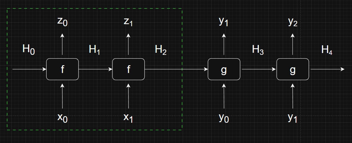
The portion that is inside the dotted green box is the encoder part of the architecture. You might have noticed that this is identical to a figure shown earlier. \( f \) is just a regular RNN that takes in the input sequence then eventually outputs a final hidden state \( H_2 \).
\( H_2 \) is then passed to the decoder part of the architecture. Another RNN \( g \) uses this hidden state and an input \( y_0 \) to generate the next element \( y_1 \). Note that input \( y_0 \) is usually just a “beginning of sequence/sentence” control token. This process is repeated to get \( y_2 \) and so on. It usually ends when \( g \) generates an “end of sequence/sentence” control token.
A popular application of the encoder-decoder is for translation. Input sequence \( X \) could be a French sentence, and the output sequence \( Y \) could be the corresponding English sentence.
The Attention Mechanism
Finally, we arrived at the attention mechanism for the Seq2seq model. Notice that in the encoder-decoder configuration figure above, only a single hidden state \( H_2 \) is passed to the decoder. For long input sequences, it was noticed that early elements at the beginning of the sequence appears to have little impact and seems to be forgotten by the final hidden state. The original paper that introduced the attention mechanism to address this issue was published all the way back in 2014!
The calculations for this section are not difficult, but there are a lot of them, and it gets messy really fast. I will only try to highlight the key points that convey the idea here instead of going over everything. If you need more, this YouTube video does a fantastic job at going over everything in a lot of detail.
Now, let’s take a look at our encoder-decoder configuration with the added attention mechanism.

The key difference is really just the inclusion of the context vectors \( c_i \). Here, the decoder RNN \( g \) uses the final hidden state \( H_2 \) from the encoder, the beginning of sequence/sentence token \( y_0 \), and the context vector \( c_0 \) to generate next token \( y_1 \). That is, instead of \( g(y_0, H_2) = y_1 \), we instead have \( g(y_0, H_2, c_0) = y_1 \).
This is all there is to the famous attention mechanism! It is just an additional context vector that helps carry information from previous tokens. Specifically, the context vector is calculated from the previous hidden states generated by the encoder model, and so the information it carries is that of the previous hidden states.
The weights \( a_i \) specifies how relevant those hidden states are and hence tell the model which parts of the input sequence to pay attention to.
The Messy Part
From the diagram, we can see that the first context vector is
What are the \( a_i \)s? This is where things get really messy. Using the notation of the YouTube video,
\( \text{align}() \) is a function that tells us how relevant hidden state \( H_i \) is to the final hidden state \( H_2 \). Essentially telling the model if it should pay attention to that particular past hidden state. Now, notice that the second context vector is
What are the \( b_i \)s? They are calculated like this:
The only difference is that instead of using the final encoder hidden state \( H_2 \), we are using the new decoder hidden state \( H_3 \). As we run the decoder, each context vector will be recalculated using subsequent new hidden states.
I warned you that this will get really complicated! Please watch the YouTube video for a complete walkthrough.