Hypothesis and A/B Testing – With a Real-World Example
Sections
- Forming a Hypothesis Then Testing It
- Randomness vs Determinism
- Control and Treatment Group
- The Sample Mean Is a Random Variable
- Central Limit Theorem
- The Test Statistic
- The Infamous P-Value
- Real World Example
Nowadays, A/B testing and randomized controlled drug trials are well known among the technically inclined. They are both examples of real-world applications of statistical hypothesis testing.
Despite their popularity, it is easy to misunderstand or forget the technical details behind hypothesis testing. This article exists so that does not happen to me! I will also show a real-world example of an A/B test that I have done in the past.
Forming a Hypothesis Then Testing It
A/B tests and randomized controlled drug trials have the same idea behind them:
-
You have a hypothesis about whether something has an effect on people.
-
You want to test if your hypothesis is correct.
-
You gather a bunch of people, try the thing on them, then see if it has an effect.
A lot of technically inclined people know about Ronald Fisher and how he invented null hypothesis testing. Based on my personal experience, few know that the modern rigorous framework of hypothesis testing was formalized by Jerzy Neyman and Egon Pearson.
Knowledge of Neyman and Pearson might be more common among those who have taken mathematical statistics courses, since theirs is the standard mathematical approach to hypothesis testing. The Neyman-Pearson lemma is also often mentioned in those courses.
There was actually an argument between Fisher and Neyman that you might find entertaining.
Randomness vs Determinism
One thing to watch out for is trying to do hypothesis testing or gather a “statistically significant” sample in deterministic situations. For example, flipping a switch to find out if it controls the lights in a room does not require any statistics!
Here is a better real-world example that I have encountered in the past: a software developer wrote a program that goes through user records to look for a specific error. This error involves a user-centric variable that keeps track of how many times the user performed a particular action. The program compared this variable with the user activity logs and produced a list of users with any mismatch.
This is a deterministic process: if the program was written correctly, users on the output list are those with a mismatch between the variable and what was in their logs. This was easy to check as well by examining a few users on that list. However, a colleague of the software developer actually wanted to do statistical sampling and hypothesis testing to check if there was actually a mismatch!
The real-world example brings up an interesting question: when do we actually do statistical sampling and hypothesis testing?
When To Do Statistical Sampling
In the framework of statistics, sampling is done to collect data points from a population. These data points are then used to calculate estimators of population characteristics. A classic example is if we want to know the average height of the USA male population but don’t have the resources to measure everyone, we could collect a random sample and calculate the sample mean.
If we have the ability to measure everyone, we can get the population average directly and do not need to construct an estimator. For the aforementioned real-world example, the computer program goes through every single user and checks for a specific error. There is no need to estimate anything.
When To Do Hypothesis Testing
Statistical hypothesis tests are a collection of highly specific statistical frameworks that involve precise mathematical assumptions. We must avoid the misconception that we can test any hypothesis we can dream of, such as the hypothesis that a light switch controls the lights in a room or the hypothesis that a software variable is bugged and mismatched with the logs.
Statistical hypothesis tests require estimators constructed using random samples taken from one or more populations. The tests are only required due to the random nature of the sampling process and the fact that a sample might not fully capture all the details of the population. There is no reason to run a statistical test when we are able to measure the entire population or if the scenario does not fit into the framework of statistical sampling.
The next sections will talk about the statistical hypothesis testing framework used in A/B testing and randomized controlled drug trials.
Control and Treatment Group
A naive approach to testing whether something has an effect on people could be just getting a group of people and then trying the thing on them. For example, if we want to test if a drug cures a disease, we could gather a group of people with the disease, get them to try the drug, and then check if they are cured of the disease.
However, we would have no idea if people in this group would have been cured of the disease if they never took the drug! Maybe a lot of them are taking another, more effective drug? Maybe their immune system would have cured them of the disease even if they never took our drug?
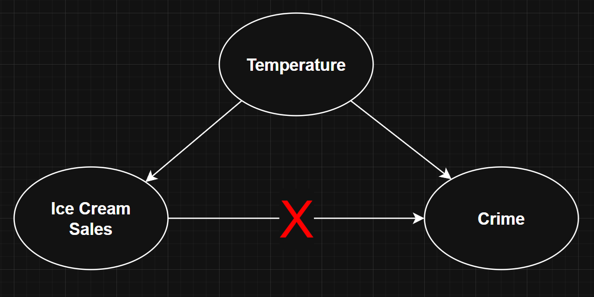
This is the issue of confounding. A lot of examples of confounding can be found on this website. A particularly famous one is how ice cream sales correlate with crime rate. The real culprit is temperature. When it gets hotter during summer weather, more people are out on the streets, causing both crime and ice cream sales to rise at the same time.
The general solution to confounding is this:
-
Gather a group of people who are as varied as possible to avoid any biases.
-
Randomly split them into a treatment group and a control group.
-
The treatment group gets the drug while the control group gets a placebo.
-
The process might be blinded, which means either the participants and/or investigators are not aware of the exact details of the experiment. Again, to avoid biases.
Strictly speaking, controlling an experiment is not an official part of the statistical hypothesis testing framework. The hypothesis test is only done because our control and treatment groups are viewed as samples from two different populations. It is a test of whether the two populations are different. For example, if the two populations have different population means. Like I mentioned in the previous section, the test is conducted due to the random nature of the sampling process and the fact that the samples might not fully capture all the details of the two populations.
Note that in the case of A/B testing, one group gets the A version while the other group gets the B version, and we want to see the difference between both versions. A/B testing is the same as the drug trial scenario if A is the drug and B is the placebo. Because of this, we will be using these two scenarios interchangeably.
The Sample Mean Is a Random Variable
Given an independent and identically distributed (IID) sample \( x = (x_1, x_2, ..., x_n ) \), the sample mean is \( \bar{x} = \sum_i x_i \). A key idea behind hypothesis testing is that the sample mean is a random variable and therefore has a probability distribution known as the sampling distribution.
The standard deviation of the sampling distribution, also known as the standard error is \( \bar{\sigma} = \frac{\sigma}{\sqrt{n}} \), where \( \sigma \) is the standard deviation of the population distribution. We can see from this quantity that the standard error falls at the rate of \( \sqrt{n} \) as sample size \( n \) increases.
If the sample is taken from a normally distributed population, the sample mean will also be normally distributed. This is not true if the sample is taken from non-normal distributions. There is no general way to tell what the sampling distribution is. That being said, we will talk about a way to try and approximate it in the next section.
Central Limit Theorem
A common form of the central limit theorem (CLT) that is well-known among the technically inclined says that
What the arrow with a d on top of it is saying is that the distribution of the random variable \( \sqrt{n}( \bar{x}_n - \mu ) \) converges to a normal distribution with mean \( 0 \) and variance \( \sigma^2 \) as sample size \( n \) goes to infinity. \( \mu \) here stands for the population mean.
There are a lot of hidden nuances with this theorem. For example, it does not say how fast the convergence is or how good the approximation is. Also, since by the law of large numbers the sample mean \( \bar{x}_n \) converges to the deterministic value of the population mean \( \mu \), we cannot say the sampling distribution of the sample mean converges to a normal distribution!
However, if we are willing to say \( \sqrt{n}( \bar{x}_n - \mu ) \sim N(0, \sigma^2) \) for large \( n \), where the \( \sim \) symbol means the random variable on the left has the probability distribution on the right, then we can sort of algebraically manipulate the approximation into
Note that for small \( n \), the Student t-distribution is used as an approximation instead. But for simplicity, we will stick to the normal distribution in this article.
The Test Statistic
So far, we have a treatment and a control group, or in the case of A/B testing, an A group and a B group. These two groups are treated as IID samples from hypothetical populations. For example, the group exposed to A is hypothetically a sample from a large population in which all the people are exposed to A.
Let \( \bar{a} \) and \( \bar{b} \) be the sample means for the A and B group respectively. Let \( \bar{x} = \bar{a} - \bar{b} \) be their difference. Imagine a population distribution of the differences between a random pairs of A and B group individuals. Then, \( \bar{x} \) is the mean of a sample taken from this population. We will assume that the A group received the drug, the B group received the placebo, and that \( \bar{x} > 0 \).
We can use the central limit theorem to get approximates \( \bar{a} \sim N(\mu_a, \sigma_a^2) \) and \( \bar{b} \sim N(\mu_b, \sigma_b^2) \). Then the approximation \( \bar{x} = \bar{a} - \bar{b} \sim N(\mu_a - \mu_b, \sigma_a^2 + \sigma_b^2) \).
\( \bar{x} \) is usually transformed into a test statistic for the hypothesis testing. The z-test statistic is
\[ z = \frac{ \bar{x} - (\mu_a - \mu_b) }{ \sqrt{ \frac{\sigma_a^2}{n_a} + \frac{\sigma_b^2}{n_b}} }. \]We will see later that we can get the value of \( (\mu_a - \mu_b) \) through our hypothesis testing assumptions. But we will need to replace the population variances \( \sigma_a^2 \) and \( \sigma_b^2 \) with the sample variances.
\[ z = \frac{ \bar{x} - (\mu_a - \mu_b) }{ \sqrt{ \frac{s_a^2}{n_a} + \frac{s_b^2}{n_b}} }. \]This definition ensures that the z statistic is normalized and is approximated by the standard normal distribution \( N(0,1) \). This is done so that the calculations in a hypothesis test is restricted to only the \( N(0,1) \) distribution.
The Infamous P-Value
Let \( \mu = \mu_a - \mu_b \) be the population mean of the distribution of differences. We want to test the null hypothesis that \( \mu = 0 \), which means there is no difference between A and B. In a drug trial, this means the drug has no effect. The alternative hypothesis can be \( \mu \neq 0 \), \( \mu > 0 \), or \( \mu < 0 \) depending on the scenario. Since we have \( \bar{x} > 0 \), we will use \( \mu > 0 \) as the alternative hypothesis.
With this setup, we can finally do the hypothesis test:
-
Assume that the null hypothesis \( \mu = 0 \) is true.
-
Calculate the probability \( p \) of getting our test statistic \( z \) or a greater value of \( z \) that is further away from \( \mu = 0 \), given that the null hypothesis is true.
-
Make a subjective decision on whether we choose to reject the null hypothesis based on the value of \( p \).
The way we have set this up is known as a one tailed test. The probability \( p \) is the infamous p-value. I labeled it “infamous” because there is so much misuse of the p-value that there is an entire Wikipedia article about it.
Real World Example
In this last section, I will walk through the hypothesis testing process step by step, using a real-world example of an A/B test that I ran. For privacy reasons, the context and the data are heavily censored. Whether this still reflects the actual real-world scenario is going to have to be a “trust me, bro” situation!
Here is the setup:
-
136 students were recruited for this experiment and randomly divided into two equal-sized groups.
-
Both groups were asked to earn points daily using an app.
-
Students in group A were sent occasional challenges with small monetary rewards to accumulate more points than what they usually get.
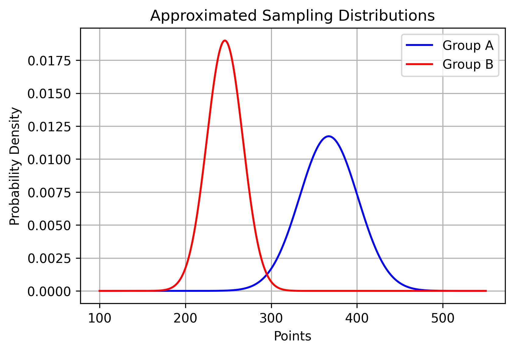
The experiment lasted 2 weeks, then the points each student collected were tallied. The sample mean and standard error of the number of points for each group are shown below. Remember that these are sample statistics because each group is treated as samples taken from larger hypothetical populations.
| Group | Mean | Standard Error |
|---|---|---|
| A | 367 | 34 |
| B | 246 | 21 |
Here is a plot showing the sampling distributions of each group approximated using the central limit theorem.
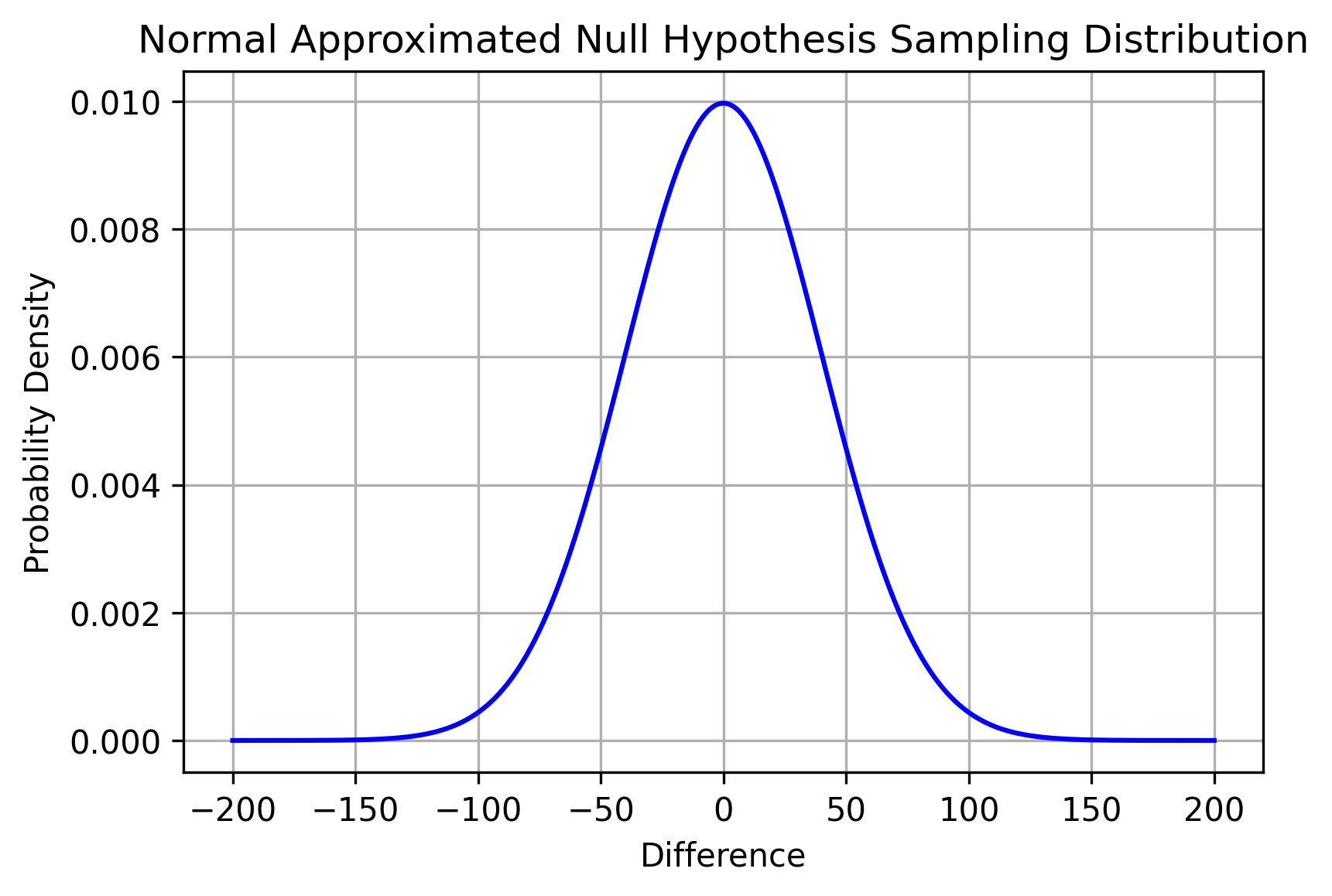
Like we said before in the previous sections, the actual sampling distribution that we are doing a hypothesis test on is the differences between group A and group B. We combine the two sample means above to get a new sample mean \( \bar{x} = \bar{a} - \bar{b} \). Using the normal approximation, we get the approximated sampling distribution as \( \bar{x} \sim N(\mu_a - \mu_b, \sigma_a^2 + \sigma_b^2) \).
Finally, if we assume the null hypothesis \( \mu = \mu_a - \mu_b = 0 \) is true, this is what the normal approximated sampling distribution of \( \bar{x} \) looks like.
Given the size of the sample groups, we performed a z-test instead of a t-test. The z-statistic is
Again, like we mentioned before in previous sections, the z-statistic is normalized so that it now has the standard normal distribution \( z \sim N(0, 1) \). \( z = 3.03 \) has a nice intepretation: if the null hypothesis is true, the test statistic we got is \( 3.03 \) standard errors from the mean. The corresponding p-value is \( p = 0.0012 \). This means that if the null hypothesis is true, the probability that we got \( z >= 3.03 \) is \( 0.12 \% \).
The p-value can be shown as a colored region on the sampling distribution. However, since the value we got is tiny, I had to cut off a big part of the plot and zoom in for us to see it.

We can think of the red region as where the sample mean we got landed assuming that the null hypothesis is true. Based on the low \( 0.12 \% \) probability of getting this sample mean and its test statistic, if the null hypothesis is true, I subjectively chose to reject the null hypothesis.
I concluded that this could be evidence that occasional challenges with small monetary rewards influenced the students in group A to collect more points.