When Not To Use Bayesian Probability Estimation

When can Bayesian methods lead to the same or similar results as simpler traditional methods? When can it be advantageous to use Bayesian methods instead of traditional ones? This is an attempt at exploring these questions for a particular scenario.

The scenario in question is taken from a 2020 Youtube video advocating for the use of Bayesian probability estimation. The video itself is based on a 2011 blog post. Their scenario goes like this: suppose we have to choose between two Amazon sellers, for the exact same product, and at the exact same price.

90% of seller B’s reviews were positive, but this is just from 20 reviews. There is more information from seller A’s 100 reviews. However, only 85% of seller A’s reviews were positive. Which seller should we choose?

The Bayesian Method

Both the Youtube video and the blog post propose that instead of just relying on the sellers’ percentage of positive reviews, we can use the Bayesian method to also take into account each seller’s total number of reviews. They assume that each seller has a fixed probability $p$ of acquiring a good review every time they sell to a customer. For example, $p_a$ is the chance that we will be satisfied enough to give sellar A a good review.

Classic statistics would use the mean $\frac{y}{n}$ as an unbiased estimator of $p$ , where $y$ is the number of positive reviews, and $n$ is the total number of reviews. This is also the maximum likelihood estimator (MLE). Formal details on these concepts, and their derivations, can be found in this set of lecture notes.

On the other hand, there are several ways to apply the Bayesian method. A common way of doing so is via this algorithm.

1. Assume that $p$ has equal probability of being any number in $(0,1)$ .
2. Use Bayes’ theorem to update this assumption.
3. Use this updated assumption to estimate the probability $p$ .

Maximum A Posteriori Estimation

Without going into too much technical details, step 1 attempts to use an uniform distribution as an uninformative prior and step 2 updates this into a beta distribution posterior. Step 2’s update of the uniform distribution in step 1 will increase in impact as we get more data. This way, the fact that seller A has much more data (number of trial) than seller B is taken into account.

Step 3 highlights the fact that, to actually make a decision between seller A and B, we need some kind of estimate of the probability $p$ . This can be done with a method like maximum a posteriori estimation (MAP). MAP is just taking the mode of the posterior distribution in step 2, which will give us the same answer as the MLE estimator $\frac{k}{n}$ .

In general, if the prior is uniform, the MAP estimator will be the same as the MLE estimator, so there is nothing extra to be gain from using the Bayesian framework this way.

Laplace’s Rule of Succession

“Laplace’s Rule Of Succession” is an alternative to using MAP in step 3. Instead of taking the mode of the posterior like for MAP, we take the mean of the posterior distribution, which is also the expected value of parameter $p$ with respect to the data. In this case, the Laplace’s Rule estimator is

The math to derive this can take a little effort, but it all boils down to starting with the usual sample mean $\frac{k}{n}.$ then simply adding a 1 to the numerator, and a 2 to the denominator.

Laplace’s Rule vs Arithmetic Mean

For large $\frac{k}{n}$ and $\frac{k}{n}$ , the difference between the Laplace’s rule estimator $\frac{k}{n}$ and the sample mean $\frac{k}{n}$ is tiny. This is not a surprise since Bayesian statistics is known to converge to the same result as traditional frequentist statistics. So, Laplace’s rule is only relevant for small samples. We can visually compare the difference between Laplace’s rule and the arithmetic mean with Python.

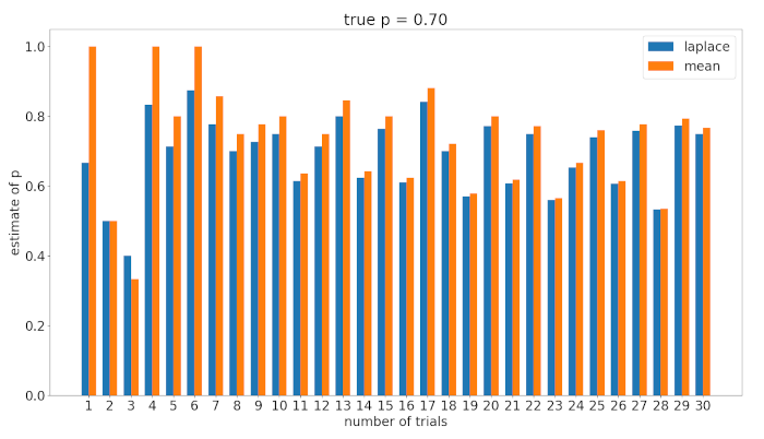
It is obvious that the difference falls off rapidly even for small increases in $n$ when plotting the difference in Python.

diff = []

for i in range(0,len(mean)):
    diff.append(abs(mean[i]-laplace[i])

plt.plot(diff)
plt.show()

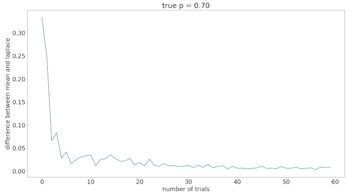
Laplace’s Rule vs Arithmetic Mean

we can see that Laplace’s rule has some form of inertia, and tend to be closer to $p=0.50$ than the arithmetic mean, by plotting the absolute distance from $p$ for each estimator.

l_dist, m_dist = [], []

for i in range(0,len(mean)):
    l_dist.append(abs(laplace[i]-0.5))
    m_dist.append(abs(mean[i]-0.5))

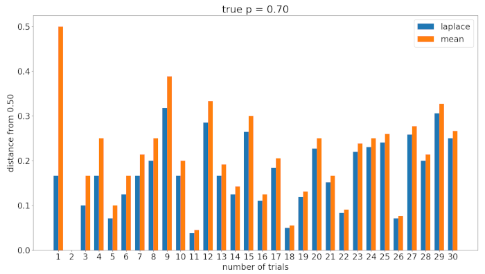
This makes sense since the Laplace’s rule estimator $\frac{k+1}{n+2}$ is equivalent to adding one success and one failure to the data. Also, this is expected behavior for a Bayesian method: we start with a prior assumption that $p$ and revise away from this assumption as data comes in.

In my humble opinion, using the Bayesian approach for this scenario does not appear advantageous over the simple sample mean. It is only relevant for small samples, and only provide a small, possibly irrelevant, shift towards $p=0.5$ .