Bias and Variance in Statistics and Machine Learning - Part 1

Bias and Variance in Statistics

Attachments

article code.txt (831 B)

In this article, I explore the concept of bias and variance, in both statistics and machine learning. These terms are derived using similar methods in both fields, but actually refer to different concepts. I will first start with how these terms are used in statistics.

I will talk about the machine learning case in part two of this article, which will also touch on the observation of a tradeoff between bias and variance in machine learning algorithms, and how such a tradeoff can be absent from modern algorithms such as neural networks and random forests

The Statistical Model

Suppose we have a set of data $ D_n = \{ x_1,...,x_n \} $ of size $ n, $ where each point $ x_i $ is drawn independently from a distribution $ P. $ I am suppressing the $ n $ in $ D_n, $ and writing it as just $ D $ to reduce clutter. Let $ y $ be some parameter of $ P $ that we wish to estimate. Let $ h_D $ be an estimator calculated from the data.

Note that I am using the non-standard notation $ h_D, $ which stands for “Hypothesis calculated from Data”. This is so that our notation is consistent with what we will be using in part 2 of this article. An example of a that is often calculated from samples would be the sample mean,

$$ h_D = \frac{1}{n} \sum_{i=1}^{n} X_i. $$

To illustrate, I will treat this set of data on public housing resale prices in Singapore as the population, from which I took a random sample of $ n = 30 $ data points.

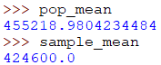
Because each data point in the sample $ D $ is randomly drawn from the population, the sample mean will vary each time we sample. For this particular draw, our sample mean was lower than the population mean.

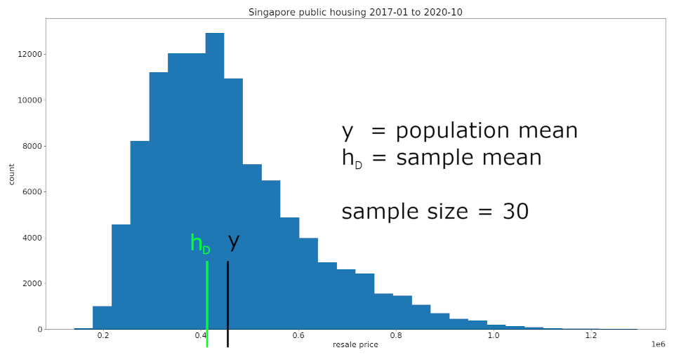
We can see that, even with just $ n = 30 $ , the sample mean is (visually) close to the population mean. The python code and data source used in this figure can be found in the article code.txt attachment located at the top of this article.

Bias of an Estimator

The bias of estimator $ h_D $ is the difference between its expected value $ \mathbb{E}[h_{D}] $ and the true parameter value $ y. $ Note that this expected value taken over all possible $ D, $ which are randomly generated sets of data with size $ n $.

$$ \text{Bias}(h_D) = \mathbb{E}[h_D - y]. $$

It is known that the sample mean is an unbiased estimator of the population mean. Which means this quantity is actually zero when $ h_{D} $ is the sample mean. However, the bias might not be zero for other estimators $ h_{D} $ .

Consistency

Note that the bias is defined here for a data set $ D $ with fixed finite size $ n $ . There is a similar concept for the estimator’s behavior as the number of data points $ n $ goes to infinity.

Of course, we would like the estimator to get closer and closer to the true parameter value as $ n $ increases. Ideally, we want to have $ h_D = y $ if we somehow managed to collect infinite number of samples. This is known as “consistency” and estimators with this property are called consistent.

Variance of an Estimator

The variance of an estimator is its expected squared difference from its own expected value,

$$ \text{Var}(h_D) = \mathbb{E}[(h_D - \mathbb{E}[h_D])^2]. $$

The variance formalizes the notion of how $ h_D $ can vary from its expected value every time we calculate it from a set of randomly sampled data $ D $ .

The variance is defined in terms of the squared difference, rather than the absolute difference. This is a paradigm that we will see everywhere in statistics and machine learning. Two possible reasons for the prevalence of this paradigm could be:

The absolute value function $ g(x) = |x| $ is not differentiable at $ x = 0 $ , but the square function is differentiate everywhere.
For a fix set of sample data $ D $ , the sample mean is the quantity that minimizes the sum of squared deviations $ \text{Var}(h_D) $ .

One thing to note is that the square function $ f(x) = x^2 $ increases exponentially in $ x $ . So, large deviations from $ y $ contributes disproportionally more to the MSE than smaller deviations.

Standard Deviation

The standard deviation is the square root of the variance. This is often used over the variance as an indicator of how much values can vary. A famous example is the 68-95-99.7 rule which estimates that 68% / 95% / 99.7% of an approximately normally distributed set of data has values within 1 / 2 / 3 standard deviations from the mean.

The Mean Square Error

The mean square error (MSE) is the expected value of the squared difference between the estimator and the parameter.

$$ \mathbb{E}[(h_D - y)^2]. $$

We can decompose the MSE into two terms, by using the “adding zero” trick to add and also subtract a $ \mathbb{E}[h_D] $ term before expanding the square.

$$ \begin{align} \mathbb{E}[(h_D - y)^2] &= \mathbb{E}[(h_D - \mathbb{E}[h_D] + \mathbb{E}[h_D] - y)^2] \\[0.5em] &= \mathbb{E}[(h_D - \mathbb{E}[h_D])^2] + (\mathbb{E}[h_D] - y)^2 \\[0.5em] &= \text{Var}(h_D) + \text{Bias}^2(h_D). \end{align} $$

The derivation is not difficult, but can get messy. Please refer to this wikipedia section for the full derivation: https://en.wikipedia.org/wiki/Mean_squared_error#Proof_of_variance_and_bias_relationship.

Stein’s Paradox

After reading my example on the sample and population mean, you might be wondering if the sample mean is the best estimator for the population mean in terms of minimizing the mean square error? Surprisingly, it turns out that the answer is “no”! An even more shocking fact is that no one knows what estimator of the population mean minimizes the mean square error!

This open problem is closely related to Stein’s Paradox. A great discussion about the history and the mystery surrounding the search for the best estimator of the population mean can be found in a classic statistics paper by Bradley Efron and Carl Morris.

So, we conclude our brief summary of bias and variance in statistics. We will look at bias and variance from a machine learning perspective, in part 2 of this article.